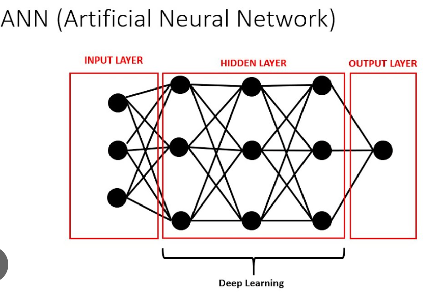
Deep studying is a subset of machine studying, which itself is a subset of synthetic intelligence (AI). Deep studying fashions are impressed by the construction and performance of the human mind and are composed of layers of synthetic neurons. These fashions are able to studying advanced patterns in knowledge by means of a course of known as coaching, the place the mannequin is iteratively adjusted to attenuate errors in its predictions.
On this weblog publish, we’ll stroll by means of the method of constructing a easy synthetic neural community (ANN) to categorise handwritten digits utilizing the MNIST dataset.

The MNIST dataset (Modified Nationwide Institute of Requirements and Know-how dataset) is without doubt one of the most well-known datasets within the area of machine studying and laptop imaginative and prescient. It consists of 70,000 grayscale photographs of handwritten digits from 0 to 9, every of measurement 28×28 pixels. The dataset is split right into a coaching set of 60,000 photographs and a take a look at set of 10,000 photographs. Every picture is labeled with the corresponding digit it represents.
We’ll use the MNIST dataset offered by the Keras library, which makes it simple to obtain and use in our mannequin.
Earlier than we begin constructing our mannequin, we have to import the mandatory libraries. These embody libraries for knowledge manipulation, visualization, and constructing our deep studying mannequin.
import numpy as np
import pandas as pd
import matplotlib.pyplot as plt
import seaborn as sns
import tensorflow as tf
from tensorflow import keras
numpyandpandasare used for numerical and knowledge manipulation.matplotlibandseabornare used for knowledge visualization.tensorflowandkerasare used for constructing and coaching the deep studying mannequin.
The MNIST dataset is out there immediately within the Keras library, making it simple to load and use.
(X_train, y_train), (X_test, y_test) = keras.datasets.mnist.load_data()
This line of code downloads the MNIST dataset and splits it into coaching and take a look at units:
X_trainandy_trainare the coaching photographs and their corresponding labels.X_testandy_testare the take a look at photographs and their corresponding labels.
Let’s check out the form of our coaching and take a look at datasets to grasp their construction.
print(X_train.form)
print(X_test.form)
print(y_train.form)
print(y_test.form)
X_train.formoutputs(60000, 28, 28), indicating there are 60,000 coaching photographs, every of measurement 28×28 pixels.X_test.formoutputs(10000, 28, 28), indicating there are 10,000 take a look at photographs, every of measurement 28×28 pixels.y_train.formoutputs(60000,), indicating there are 60,000 coaching labels.- `y_test
.formoutputs(10000,)`, indicating there are 10,000 take a look at labels.
To get a greater understanding, let’s visualize one of many coaching photographs and its corresponding label.
plt.imshow(X_train[2], cmap='grey')
plt.present()
print(y_train[2])

plt.imshow(X_train[2], cmap='grey')shows the third picture within the coaching set in grayscale.plt.present()renders the picture.print(y_train[2])outputs the label for the third picture, which is the digit the picture represents.

Pixel values within the photographs vary from 0 to 255. To enhance the efficiency of our neural community, we rescale these values to the vary [0, 1].
X_train = X_train / 255
X_test = X_test / 255
This normalization helps the neural community be taught extra effectively by making certain that the enter values are in an identical vary.
Our neural community expects the enter to be a flat vector slightly than a 2D picture. Subsequently, we reshape our coaching and take a look at datasets accordingly.
X_train = X_train.reshape(len(X_train), 28 * 28)
X_test = X_test.reshape(len(X_test), 28 * 28)
X_train.reshape(len(X_train), 28 * 28)reshapes the coaching set from (60000, 28, 28) to (60000, 784), flattening every 28×28 picture right into a 784-dimensional vector.- Equally,
X_test.reshape(len(X_test), 28 * 28)reshapes the take a look at set from (10000, 28, 28) to (10000, 784).
We’ll construct a easy neural community with one enter layer and one output layer. The enter layer could have 784 neurons (one for every pixel), and the output layer could have 10 neurons (one for every digit).
ANN1 = keras.Sequential([
keras.layers.Dense(10, input_shape=(784,), activation='sigmoid')
])
keras.Sequential()creates a sequential mannequin, which is a linear stack of layers.keras.layers.Dense(10, input_shape=(784,), activation='sigmoid')provides a dense (absolutely linked) layer with 10 neurons, enter form of 784, and sigmoid activation operate.
Subsequent, we compile our mannequin by specifying the optimizer, loss operate, and metrics.
ANN1.compile(optimizer='adam', loss='sparse_categorical_crossentropy', metrics=['accuracy'])
optimizer='adam'specifies the Adam optimizer, which is an adaptive studying price optimization algorithm.loss='sparse_categorical_crossentropy'specifies the loss operate, which is appropriate for multi-class classification issues.metrics=['accuracy']specifies that we wish to observe accuracy throughout coaching.
We then prepare the mannequin on the coaching knowledge.
ANN1.match(X_train, y_train, epochs=5)
ANN1.match(X_train, y_train, epochs=5)trains the mannequin for five epochs. An epoch is one full cross by means of the coaching knowledge.

After coaching the mannequin, we consider its efficiency on the take a look at knowledge.
ANN1.consider(X_test, y_test)
ANN1.consider(X_test, y_test)evaluates the mannequin on the take a look at knowledge and returns the loss worth and metrics specified throughout compilation.

We are able to use our educated mannequin to make predictions on the take a look at knowledge.
y_predicted = ANN1.predict(X_test)
ANN1.predict(X_test)generates predictions for the take a look at photographs.

To see the expected label for the primary take a look at picture:
print(np.argmax(y_predicted[10]))
print(y_test[10])
np.argmax(y_predicted[10])returns the index of the best worth within the prediction vector, which corresponds to the expected digit.print(y_test[10])prints the precise label of the primary take a look at picture for comparability.

To enhance our mannequin, we add a hidden layer with 150 neurons and use the ReLU activation operate, which frequently performs higher in deep studying fashions.
ANN2 = keras.Sequential([
keras.layers.Dense(150, input_shape=(784,), activation='relu'),
keras.layers.Dense(10, activation='sigmoid')
])
keras.layers.Dense(150, input_shape=(784,), activation='relu')provides a dense hidden layer with 150 neurons and ReLU activation operate.
We compile and prepare the improved mannequin in the identical approach.
ANN2.compile(optimizer='adam', loss='sparse_categorical_crossentropy', metrics=['accuracy'])
ANN2.match(X_train, y_train, epochs=5)

We consider the efficiency of our improved mannequin on the take a look at knowledge.
ANN2.consider(X_test, y_test)

To get a greater understanding of how our mannequin performs, we will create a confusion matrix.
y_predicted2 = ANN2.predict(X_test)
y_predicted_labels2 = [np.argmax(i) for i in y_predicted2]
y_predicted2 = ANN2.predict(X_test)generates predictions for the take a look at photographs.y_predicted_labels2 = [np.argmax(i) for i in y_predicted2]converts the prediction vectors to label indices.
We then create the confusion matrix and visualize it.
cm = tf.math.confusion_matrix(labels=y_test, predictions=y_predicted_labels2)
plt.determine(figsize=(10, 7))
sns.heatmap(cm, annot=True, fmt='d')
plt.xlabel("Predicted")
plt.ylabel("Precise")
plt.present()
tf.math.confusion_matrix(labels=y_test, predictions=y_predicted_labels2)generates the confusion matrix.sns.heatmap(cm, annot=True, fmt='d')visualizes the confusion matrix with annotations.


On this weblog publish, we lined the fundamentals of deep studying and walked by means of the steps of constructing, coaching, and evaluating a easy ANN mannequin utilizing the MNIST dataset. We additionally improved the mannequin by including a hidden layer and utilizing a special activation operate. Deep studying fashions, although seemingly advanced, may be constructed and understood step-by-step, enabling us to sort out numerous machine studying issues.